Computer Vision Defect Detection, Concept to Production

TLDR

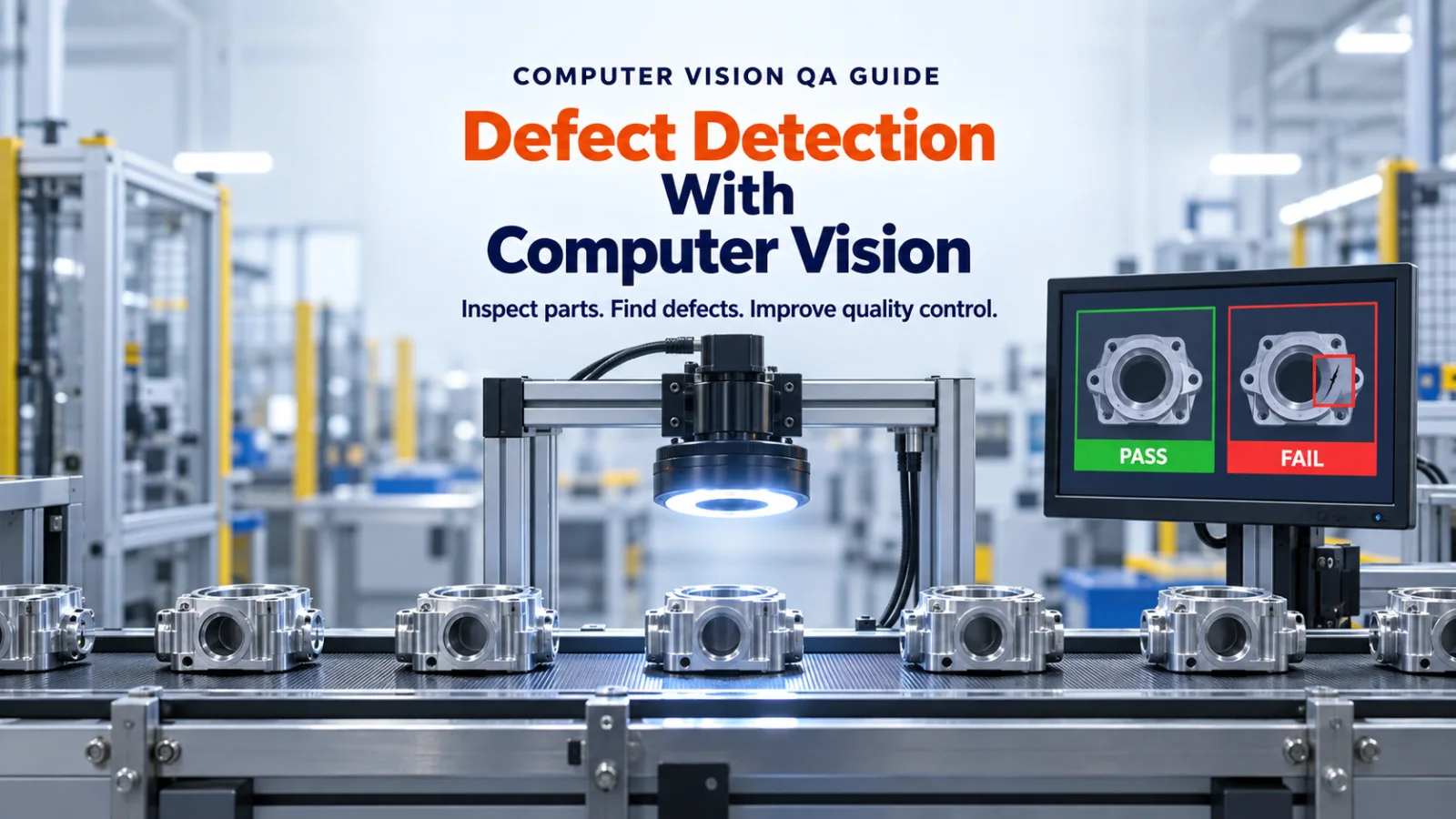
• Computer vision defect detection uses cameras, controlled lighting, and trained models to identify flaws in products or materials at line rate.
• The engineering discipline separates into five working parts. Capture, preprocessing, inference, routing, action.
• The factory integration sits underneath the pipeline. PLC triggers, image queues, worker pools, physical reject mechanisms, dashboards, and recipe switching for product variants.
• Six algorithm families cover most of the space. Rule based image processing, supervised classification, object detection, segmentation, anomaly detection, and two stage systems.
• Model choice is a second order decision. Imaging discipline and annotated corpus quality decide accuracy more consistently than model architecture does.
• Camera math runs the other direction from the model. Define the smallest defect the operator wants surfaced, decide how many pixels must cover it, then work back to sensor resolution, lens, working distance, and lighting.
• Accuracy is a misleading headline metric when defects are rare. Precision, recall, F1, mAP, IoU, and false alarms per 1,000 parts tell the actual story.
• Buy versus build is a real decision. Industrial vision platforms fit bounded rule based inspection well. Custom fine tuned models fit domain specific defects better. Hybrid setups are common.
• Detection is the start of the value chain. The corrective action loop through SPC methods turns detection data into process improvement.

The rest of this read explains each of these points with the vocabulary an engineering reader needs to make good decisions about a defect detection program.

What Computer Vision Defect Detection Actually Is

Computer vision defect detection uses cameras, controlled lighting, image processing, and trained models to identify flaws in products or materials against a defined standard. A camera captures the frame. A preprocessing step normalizes and prepares the image. A model or set of models reads the prepared frame and produces a finding, typically as a label, a bounding region, a confidence score, and where relevant a severity token. A routing rule sends the finding to an automated action, a human reviewer, or a retake queue.

The productive framing for manufacturing is direct. Vision inspection replaces sampling with continuous inspection. A human operator working sampling based manufacturing quality inspection reviews some fraction of units, typically well under 10 per cent, and infers the rest of the population from that sample. A vision system inspects every unit that passes the camera. The economic shift is a step change in coverage across every unit that passes the camera.

Two second order shifts follow from the first coverage shift.

• Consistency. Inspection stops depending on operator fatigue and shift handovers, since the model reads every frame the same way.
• Objectivity. Every finding carries a category label, a confidence score, and a source frame that can be reviewed later.

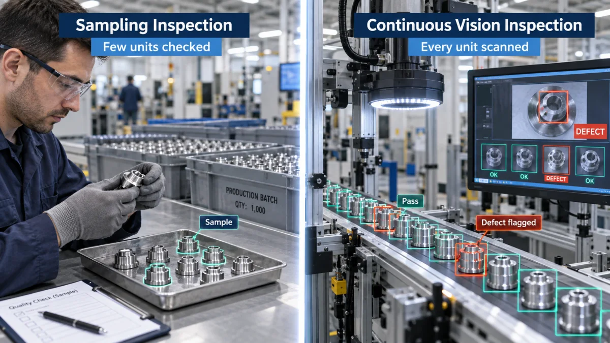
Fig 1 – Sampling Inspection Versus Continuous Inspection

The definition sets the scope. The engineering discipline sits inside a specific structure that carries the frame from the camera to the operator action, and that structure decides more of the outcome than the model choice does.

The Five Working Parts of a Defect Detection Pipeline

A production system separates into five working parts. Each part carries its own engineering discipline and a bounded interface to the parts around it. Treating them as one undifferentiated system is a common failure mode. Treating them as five separable disciplines with clean contracts between them is how programs reach production without falling over in the first quarter.

Each part in more depth.

Capture is the camera, the lens, the exposure, and the angle. This is the frame the model actually sees. Every downstream decision inherits the constraints of what capture recorded.

Preprocessing normalizes the frame before inference. Exposure normalization, orientation correction, background segmentation, and white balance correction run here. Where the setup involves multiple views or product orientations, preprocessing also selects which frames are eligible for downstream inference and which route to retake.

Inference is the model or set of models. Output shape depends on the algorithm family. A classifier produces a whole frame label. A detector produces per instance bounding regions and category labels. A segmentation model produces pixel level masks. An anomaly detector produces per region deviation scores. In every case, output carries a confidence value.

Routing applies threshold rules to the inference output. High confidence findings route to automated action. Lower confidence findings route to human review. Retake candidates route back to capture. The threshold values are a calibration decision that continues across the life of the system.

Action is the integration point with the physical line or the operator system. Reject a unit, flag it for rework, alert the operator, log the finding to a quality register, halt the line. Action carries the pipeline’s business impact.

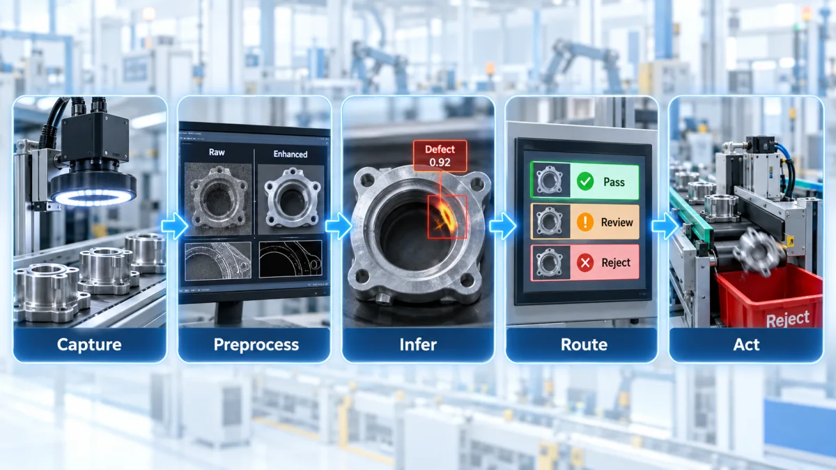
Fig 2 – The Five Working Parts of a Defect Detection Pipeline

The separation has a practical consequence for engineering teams. A model output that carries a category label, a confidence score, and a severity token should keep those three signals in different fields. A downstream decision or a presentation choice made from folded signals will get read back later as a physical severity claim, and the correction cost of that read runs high.

The five part pipeline describes the data flow. Underneath it sits the factory integration that carries the physical signals a real line produces and consumes.

The Factory Integration

A defect detection pipeline on a production line integrates with hardware and control systems that the model architecture diagram does not show. Engineering teams that skip this integration end up with a working model and a system that does not survive the first shift.

Capture Trigger From the Control System

Cameras rarely run continuously in production. A programmable logic controller (PLC) sends a trigger to the camera when a part reaches the inspection position, based on an encoder pulse, a photoelectric sensor, or a timing signal off the conveyor. The camera captures on the trigger and returns the frame with a part identifier attached. This ties every image to a specific physical unit, which the downstream routing needs to reject the correct part later.

Image Queue and Worker Pool

Frames enter a queue between the camera and inference. The queue absorbs burst rates at line speed, so a temporary inference slowdown does not drop images. A worker pool consumes the queue and runs inference. Worker count matches the sustained frame rate the line produces, with headroom for burst absorption. Queue depth monitoring surfaces slowdowns early, before the pipeline starts dropping frames or holding up the line.

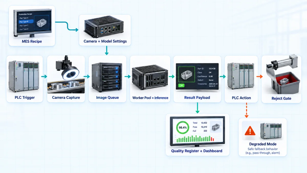
Fig 3 – The Factory Integration

Result Contract Back to the Control System

Inference produces a structured result that the PLC reads and acts on. A common shape is a JSON payload containing the part identifier, an overall pass or fail decision, per finding category and severity, confidence values, and a source frame reference. The PLC reads the payload against its own timing constraints and triggers the physical action. A parallel write goes to the quality register database for the dashboard and the corrective action loop covered later in this read.

Physical Reject Mechanism

The reject action is a physical actuator on the line. Pneumatic reject blades push a failed unit into a reject bin. Diverter arms route a failed unit to a rework conveyor. Robotic pick and place lifts a failed unit out of the flow. Halt and alert stops the line and calls the operator when the failure mode indicates a systemic issue. Each mechanism has its own timing tolerance from the inference decision to the physical action, which sets the acceptable end to end latency for the pipeline.

Dashboards and the Quality Register

Every finding writes to a quality register that carries the part identifier, the model output, the physical action taken, the timestamp, the shift, the batch, the product variant, and the machine or supplier identifier where relevant. Dashboards read the register and present per hour, per shift, per batch, per machine, and per supplier views. The dashboard carries the connective tissue between detection and corrective action, which the closing sections cover.

Recipe Switching for Product Variants

Most production lines run more than one product variant. A shift may run three or four SKUs across an eight hour block. Each variant has its own regions of interest, defect categories, thresholds, and often its own trained model. The pipeline handles this through a recipe surface. When the PLC broadcasts a new variant identifier (or an MES schedule advances to the next run), the pipeline loads the recipe for that variant. Regions of interest shift. Thresholds shift. The active model version shifts. Recipe switching happens without pipeline restart, which lets the line run continuously across variant changes.

Degraded Mode Behavior

Inference outages happen. Networks drop. Worker nodes fail. Model serving processes crash on a bad frame. Production lines do not stop for these events, and the pipeline should not force them to. Degraded mode routes the line to a defined fallback while inference is unavailable. The fallback is a business decision that the operations team owns.

Common fallback shapes include:

• Manual sampling with a logged flag indicating the affected window.
• Bypass with post shift review, marking the affected units for review after the outage window closes.
• Line halt where the defect risk is high enough to justify the throughput loss.

Whichever choice the operations team makes for the specific product and defect class, the pipeline honors it, logs the affected window, and reprocesses queued images once inference returns.

The factory integration decides whether the pipeline survives contact with a real production line. With that integration in place, the choice of algorithm inside the inference step becomes a meaningful engineering decision.

Algorithm Approaches, and What Each Is Good For

Six algorithm families cover most of the visual defect detection space. The choice among them follows from the character of the defect and the data available for training.

Each family in more depth.

Rule based image processing applies thresholds, edge detection, contour matching, color checks, or geometric measurements to the frame using classical OpenCV operations. A stable geometry or color check produces an entirely defensible engineering result when the defect matches the rule. Reaching for a neural model where a threshold suffices is a failure of engineering judgment. Good candidates for rule based image processing include fill level checks, alignment measurements, presence and absence checks for known components, and color deviation against a specification. Industrial vision platforms such as Cognex In-Sight implement this approach against golden part references for scratches, nicks, stains, chips, missing edges, and print flaws.

Supervised classification trains a convolutional network to label whole frames or crops as good, defective, or defective in a specific category. The approach fits well where the taxonomy is bounded and enough labeled examples exist for each category. A ResNet or similar backbone fine tuned on the client’s own imagery produces reasonable results within a well scoped labeling program. Supervised classification does not localize the defect. It labels the frame.

Object detection trains a detector to produce per instance bounding regions and category labels. YOLO class detectors are common in production for their inference speed. RT-DETR and other transformer detectors carry higher accuracy at the cost of inference time. The approach fits well when the defect has a visible shape and position that matters to the downstream action.

Segmentation trains a model to produce pixel level masks of defect regions. U-Net and its descendants are the common architecture family. The approach fits well for scratches, coating defects, stains, cracks, weave defects, and print defects, where the area and shape of the defect region carries the downstream decision.

Anomaly detection learns the appearance of normal product from a corpus of good samples and flags deviations from that learned distribution. MVTec’s overview of industrial anomaly detection covers the approach applied to PCB, semiconductor, and surface inspection contexts, and the MVTec AD benchmark dataset is the current standard for evaluating industrial anomaly detection methods against pixel precise defect annotations. PatchCore and PaDiM are current strong methods. Autoencoder based approaches also apply. The approach is the right default when defect examples are rare, which describes most manufacturing programs in the first year. The output is a per region deviation score.

Two stage systems run anomaly detection to catch suspicious regions and then run a smaller supervised classifier on those regions to reduce false positives. The architecture separates the recall problem from the precision problem, which lets each stage be tuned against its own metric. Two stage systems are the right choice when false positive rates from a single stage anomaly detector run too high for the operator to trust the alerts.

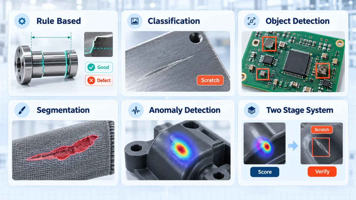
Fig 4 – Six Algorithm Families and Their Output Shapes

Architectural note. Clixlogix’s engagement on an Australian property inspection SaaS used a detection model that produced category, confidence, and severity as three separated per instance signals, with a downstream fine tuned classifier reading detected region crops and producing the reporting status. The two model architecture separated presentation weight from physical severity claims. The alternative, folding severity and presentation into a single detector output, produces the class of error that gets systems pulled from production once operators lose confidence in the alerts. The engineering choice is worth naming early in a program.

Six approaches cover the space. The choice among them follows from the shape of the problem.

Choosing an Approach

A decision framework fits inside one short section. The character of the defect and the data on hand together decide the algorithm family.

• Few or no defect examples available. Start with anomaly detection.
• Many labeled examples across a bounded taxonomy. Supervised classification or object detection.
• Location and area of the defect matter to the downstream action. Segmentation.
• Line rate is the binding constraint. Balance resolution, model size, and inference hardware before model architecture.
• Stable geometry or color rule fits the defect. Classical image processing first.
• False positive rate is the metric operators cite when talking about the system. Two stage.

The sparse defect tradeoff. When only a handful of examples exist per defect class, forcing a multi class model to learn the fine grained taxonomy on that data produces unreliable per class recall. A more defensible sequence is to solve the binary problem first with anomaly detection or a binary classifier, route flagged frames to human review, and let the reviewer assign the category label. As real defect volume accumulates, the labeled examples support a downstream multi class classifier without the cold start problem the direct multi class approach carries.

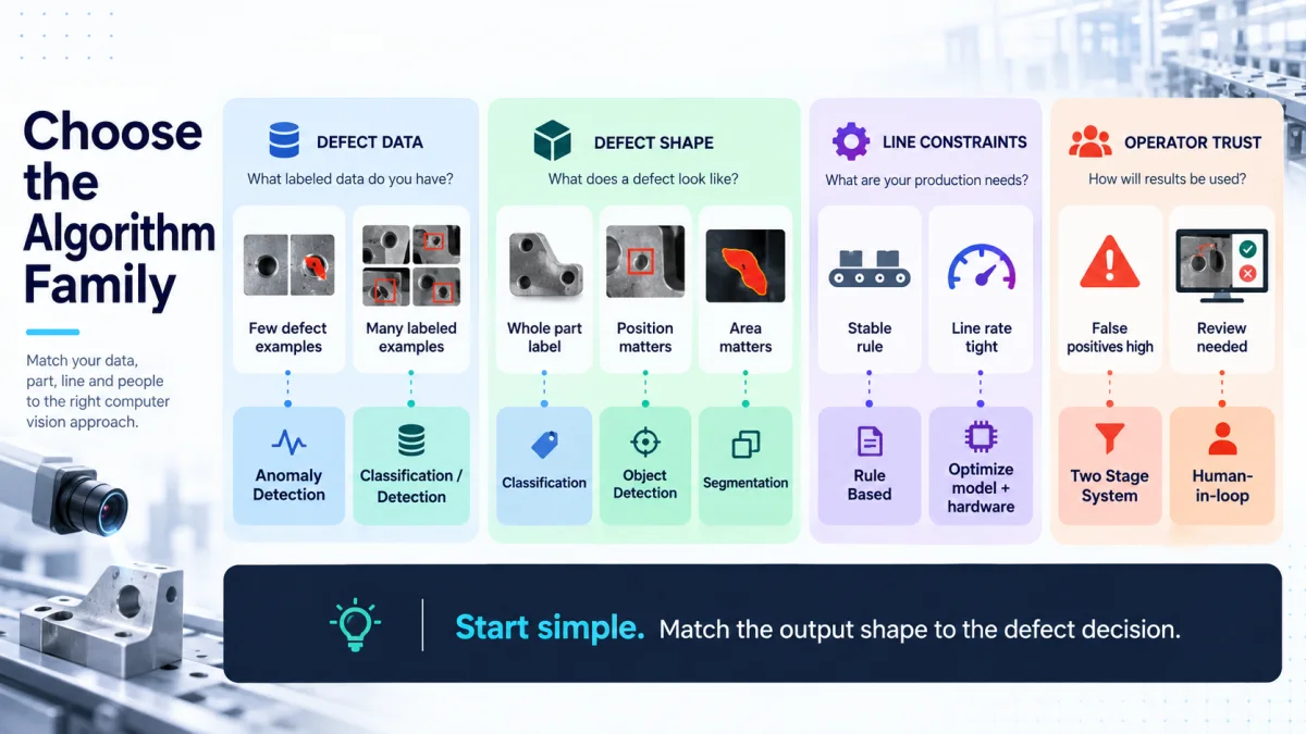
Fig 5 – Routing From Defect Character to Algorithm Family

The framework decides where a program starts. The next section decides how well any of those starts actually works.

Data and Imaging, Which Decide the Outcome

Model outcomes in visual defect detection are decided by the representativeness of the training data and the discipline of the imaging setup. This finding recurs across Clixlogix delivery engagements and across published production practice in the space.

Custom Annotated Corpora Over Public Datasets and Synthetic Imagery

A public dataset does not match the lighting, angle, and camera profile of the specific production environment. Training on that data produces a model that reads well on the public distribution and reads poorly on the line. The Australian inspection engagement rejected this shortcut and produced a training corpus of around 120,000 photos with more than 350,000 individually labeled defect instances against a versioned taxonomy. The Northern European salvage vehicle auction engagement trained on adjuster labeled data from the client’s own capture stream. Documented provenance of the training corpus becomes a defensible answer to enterprise buyers and auditors, and matters at any audit context the finding enters later.

Synthetic imagery carries its own failure modes worth naming. Copy paste augmentation, where a defect crop is transplanted onto a good sample, teaches the model to lock onto the pasted edge signature and the lighting mismatch at the paste boundary alongside the actual defect features. Diffusion generated defects introduce diffusion artifacts that the model can learn as defect features, and those artifacts do not appear in real production frames. Synthetic data can supplement a training set where the augmentation preserves realism and the artifacts are actively controlled. The validation set stays 100 per cent real regardless, so the reported accuracy reflects performance on the actual distribution the deployed system will see.

Labeling Programs Are First Class Deliverables

A detection model trains against per instance bounding regions, category labels from a defined taxonomy, and severity tokens. These do not exist in a normal manufacturing archive by default. A serious program funds a labeling program as a first class deliverable.

Two labeling channels commonly combine. A curated internal team drawn from experienced inspectors or quality engineers handles the categories with the highest downstream cost of error and the definitional judgment calls. External annotation partners cover the categories where the definitional boundary is clear enough for a well briefed external labeler to produce reliable output. A senior inspector reviewer sets the definitional boundaries between condition impacting and cosmetic only findings, and reviews a rolling sample from both channels before labels enter the training set. Where a category shows low agreement between labelers, the taxonomy definition itself gets reviewed before those labels enter training.

Fig 6 – Labeling Program Structure

Camera Math Runs Backwards From the Defect

Camera and lens selection start with the defect. The sequence has four steps that hold across every program.

1. Smallest defect size, measured on the product in millimetres. A quality specification typically names this. If it does not, an operator conversation surfaces it quickly.
2. Minimum pixel coverage per defect. Detection models produce reliable outputs when the smallest defect covers at least 3 to 5 pixels on the shortest axis. Segmentation models often need more, closer to 8 to 10 pixels, for a stable mask. Rule based checks can work with fewer pixels but only for high contrast features.
3. Pixels per millimetre the sensor must deliver at the working distance. This falls out of the required pixel coverage divided by the smallest defect size. A 0.5 mm defect that must be covered by 5 pixels requires 10 pixels per mm at the working distance.
4. Sensor resolution and field of view combination that delivers the pixels per millimetre. Field of view is the width of the product surface the camera captures in one frame. Sensor resolution divided by field of view gives pixels per mm. A 5 megapixel sensor with a 2448 pixel wide readout, capturing a 244 mm wide field of view, delivers 10 pixels per mm and meets the requirement. A wider field of view at the same sensor resolution falls below the requirement and misses the defect.

Lens selection and working distance work from field of view, sensor size, and lens focal length together. Lighting selection works from the required exposure at the frame rate the line requires, which sets the strobe intensity and duration.

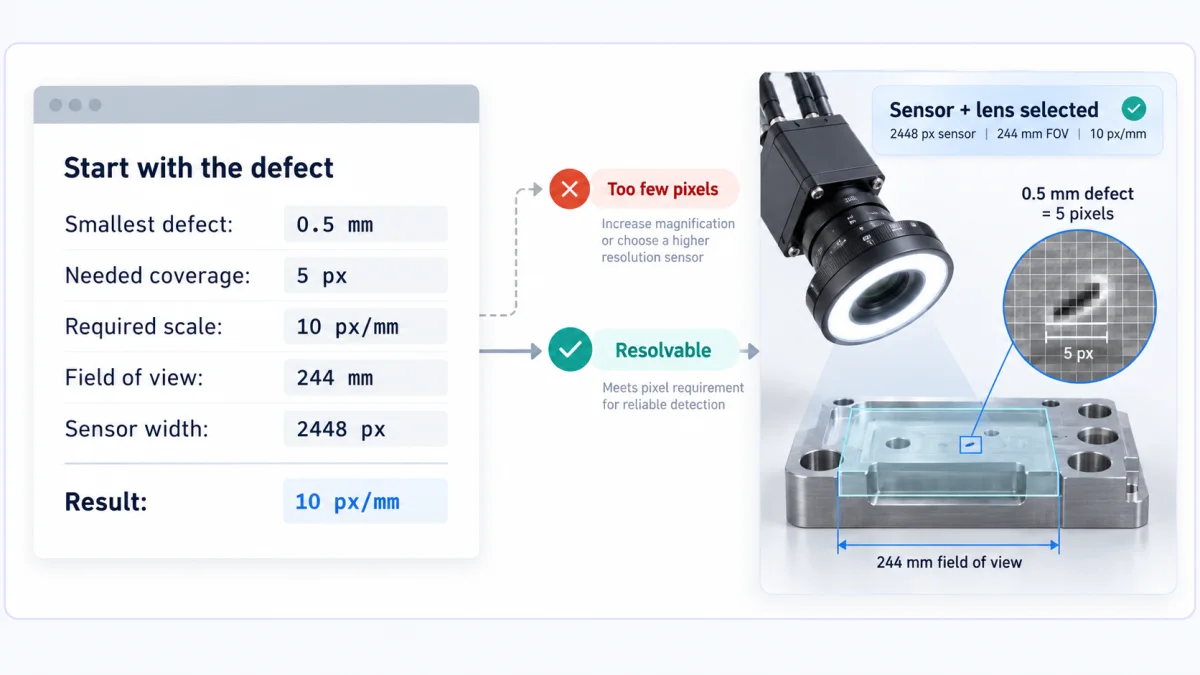
Fig 7 – Camera Math From Defect to Sensor Choice

Getting the math wrong at this step compounds through every subsequent decision. Model accuracy on a defect the camera physically cannot resolve is capped at zero, and no model architecture or training corpus recovers the missing pixels.

Area Scan Versus Line Scan Cameras

Two camera architectures serve different production geometries. The choice runs off the product shape and the line motion.

Keyence’s line scan technology overview covers the target surface types line scan handles well, including scratches, dirt, and dents on webs, sheets, and cylindrical surfaces.

Line scan setups carry different engineering considerations than area scan. Encoder synchronization drives frame geometry. Lighting must be uniform across the full line width. Line scan cameras produce very long frames that inference pipelines process in overlapping windows. Choosing line scan where area scan would work adds unnecessary complexity, and choosing area scan on a continuous web produces frames with unusable geometry.

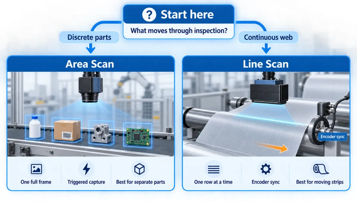
Fig 8 – Area Scan and Line Scan Camera Architectures

Imaging Discipline Decides What the Model Can Read

Industrial imaging tradeoffs deserve engineering attention early in a program. Industrial cameras carry consistent color reproduction and calibrated exposure that consumer cameras do not. Global shutter cameras hold moving product frames without motion blur, where rolling shutter cameras distort the image. External strobe lighting freezes motion at the camera, which lets the model read a sharp frame even at line speed. Basler’s lighting guide and illumination documentation cover the illumination geometry, strobe control, and camera synchronization decisions that decide contrast on different surface types, including dark field, bright field, dome, and backlight setups. Camera position, distance, and angle stay constant across shifts, batches, and suppliers, since a variable capture setup teaches the model to expect variation that the deployed system will not receive.

Reflective, curved, glossy, and textured surfaces produce specific capture problems that get tested early or get discovered too late. Chrome, painted metal, glass, glossy polymer, and wet product all reflect light in ways that read to the detector as apparent features. The salvage vision engagement handled reflective wet tarmac through background segmentation that removed the ground reflection before the detector saw the frame, and handled low sun angle glare on chrome and paint through adaptive exposure normalization with retake routing for frames past a reflection threshold.

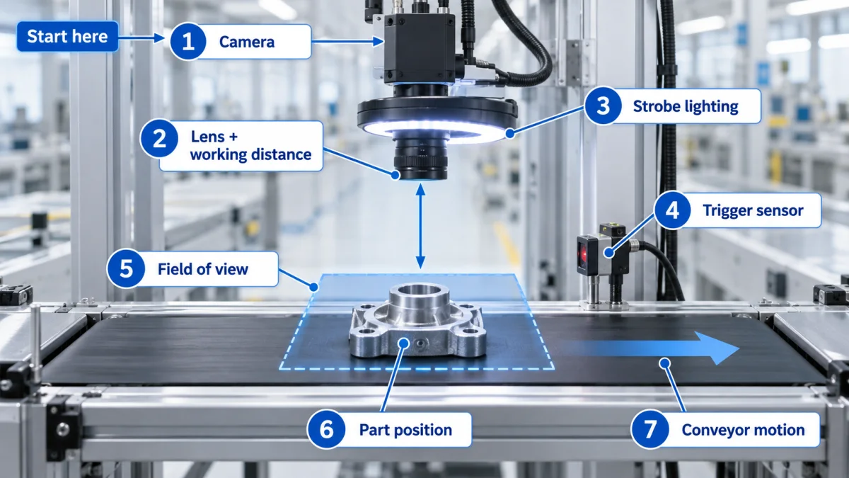
Fig 9 – Industrial Imaging Setup

Hard Negatives Reduce False Positive Rates More Reliably Than Model Tuning Does

A hard negative is a sample that looks like a defect but is not one. A shadow that looks like a stain. A packaging film reflection that looks like a scratch. A harmless surface variation that visually resembles a real crack. Adding confirmed hard negatives to the training set with explicit non defect labels teaches the model the boundary between defect and non defect at the visually ambiguous cases, which is where false positives concentrate. The result outperforms model tuning as a false positive reduction strategy, because model tuning without hard negatives moves the decision boundary blindly.

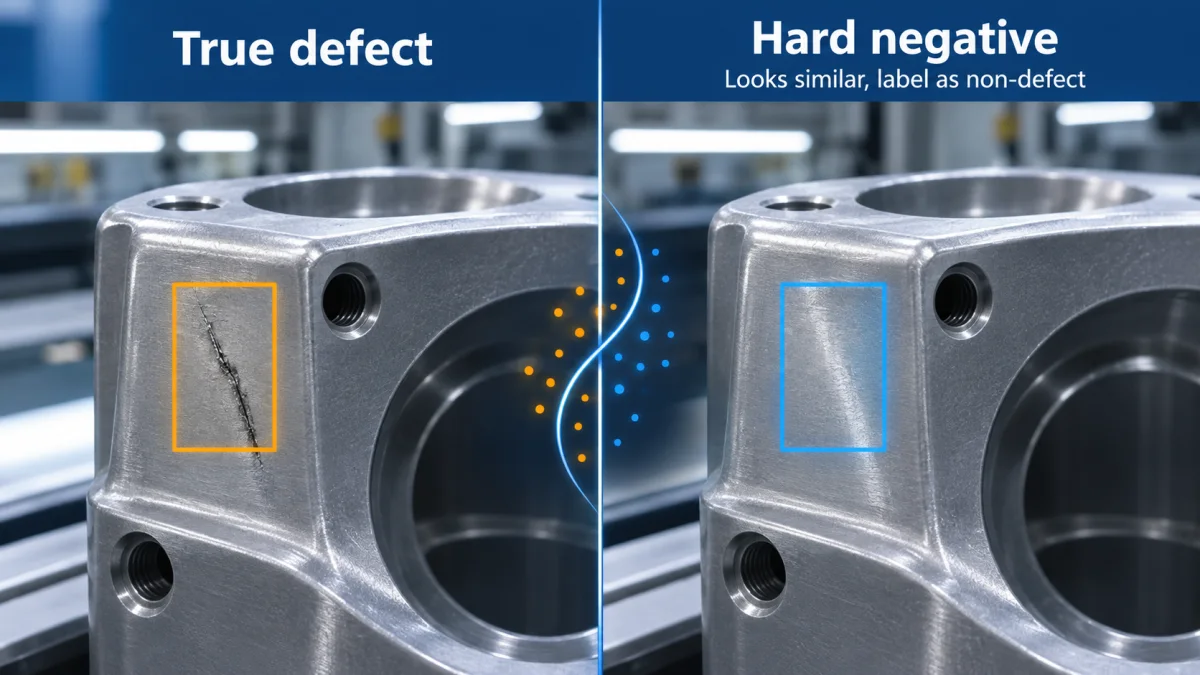
Fig 10 – Hard Negatives Teach the Boundary

Data and imaging carry the accuracy floor. Production adds a second set of decisions that decide whether the accuracy holds under real load.

Production Considerations

A model that clears its held out validation set has not yet cleared production. Six production considerations sit between the validation set and a working line integration.

• Takt time and inference latency. Takt time is the interval between successive units leaving the line. If the line produces 100 units per minute, takt time is 600 milliseconds per unit. Inference latency has to fit inside takt time, minus the time needed for capture, preprocessing, routing, and physical action. Four separate latency measurements deserve tracking. Single image inference latency measures how long the model takes on one frame in isolation. End to end inspection time measures capture to physical action, which includes preprocessing, model inference, routing, and actuator response. Sustained throughput measures how many frames the pipeline handles per second across a long window, which surfaces queue backpressure and warm cache effects. Cold start latency measures the first inference after a model load or a container restart, which sets the minimum interval before which a recipe change can bring the model into service. Runtime documentation from vendors such as the NVIDIA TensorRT optimization guide covers the batching, precision mode, and profiling techniques that separate the four latency measurements at the hardware level. A pipeline that hits its single image target and fails on sustained throughput will not survive a full shift.

• Edge versus cloud inference. Deterministic latency and physical line control favor edge inference on hardware close to the camera. Iteration velocity, model management, and access to larger models favor cloud inference. Hybrid setups are common, where the fast path runs on edge and a suspicious fraction routes to cloud for deeper analysis.

• Confidence thresholding. Every model output carries a confidence score. Every threshold decision routes the finding into one of three buckets. Automated action for confident findings above the high threshold. Human review for findings between the two thresholds. Retake or reject for findings below the low threshold or with poor capture quality.

• Human review gate placement. Gate placement decides the accuracy outcome. The Australian inspection engagement documented this directly. Reviewing a completed report at the end of an inspection defaulted to scanning behavior, and reviewers missed subtler errors that required them to remember what the physical evidence actually looked like earlier in the walkthrough. Moving the gate to the room level, where the reviewer sees the model output next to the physical evidence before moving on, changed the accuracy floor of finished reports. The equivalent in manufacturing quality inspection is a review station at the inspection point.

• Feedback loops. Reviewer corrections in defined categories feed the next model version through a curated training data flow. The distinction between an approval and a correction matters. An approval is an operational event. A correction is a training annotation. Folding both into the training set poisons the label distribution with signals that were never intended as labels.

• Shadow evaluation and threshold promotion. New model versions and new threshold values run in shadow mode against production traffic before they change deployed behavior. The shadow output runs alongside the live output, and the operations team compares outcomes before promoting the change. Both Clixlogix vision engagements used this practice as the standard threshold and model promotion path.

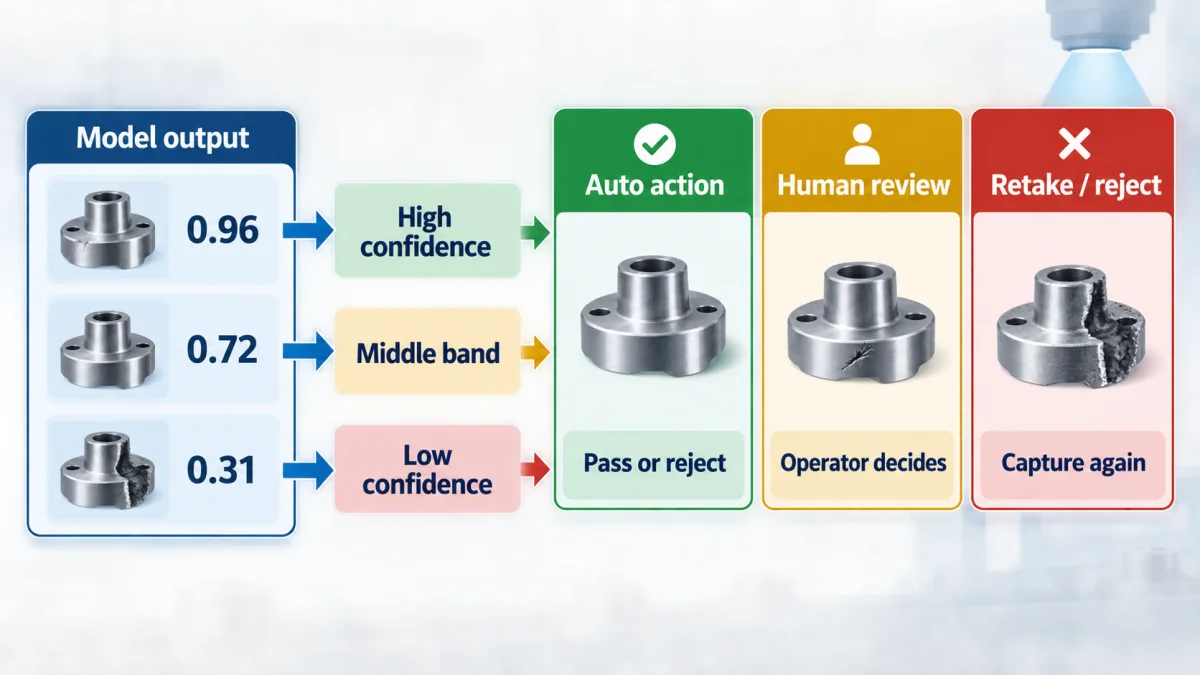
Fig 11 – Confidence Score Routing Into Three Action Buckets

Metrics That Actually Track Program Health

Accuracy is a misleading headline metric on defect detection programs where defects are rare. Six metrics carry the actual signal.

Each metric in more depth.

Precision measures, of the findings the model flagged as defects, what fraction were real defects. A precision of 0.85 means 85 per cent of alerts are true positives and 15 per cent are false alarms.

Recall measures, of the real defects that passed the camera, what fraction the model caught. A recall of 0.90 means the model caught 90 per cent of real defects and missed 10 per cent. Missed defects reach the customer.

F1 score is the harmonic mean of precision and recall, useful as a single summary when the two metrics need to move together.

Mean average precision (mAP) and intersection over union (IoU) apply to object detection and segmentation models. mAP summarizes precision across recall levels. IoU measures how well the predicted region overlaps with the ground truth region. Both belong in the evaluation report for detection and segmentation programs.

False alarms per 1,000 inspected parts is the metric operators cite in the break room. It sets whether the alerting is trustable in daily use or whether operators start ignoring the alerts. A pipeline with strong recall and a false alarm rate the operators trust survives. A pipeline with strong recall and a false alarm rate that erodes operator trust gets bypassed within a quarter.

Cost weighted false rejects and false accepts convert the raw counts into economic terms. A false reject scraps a good unit. A false accept ships a bad unit. The cost of each is not equal. The cost weighted metric supports the threshold calibration decisions the operations team makes across the life of the system.

The accuracy trap. A line running at a 1 per cent defect rate rewards a model that predicts “no defect” on every frame with 99 per cent accuracy, and that model catches zero defects. The metric that reads high tells the operator nothing about whether the system works.

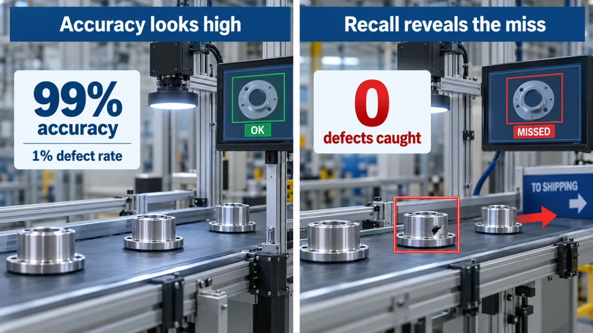
Fig 12 – Why Accuracy Alone Misleads on Rare Defect Lines

A production system that clears the initial cutover meets its next set of tests in the field. And before that field test, one decision often sits above every other. Whether to buy the system or build it.

Buy Versus Build

Industrial vision has a mature commercial platform ecosystem. Cognex, Keyence, and MVTec HALCON all serve production defect detection at scale, with hardware, software, and integration support. Custom fine tuned models on general purpose infrastructure serve a different set of problems.

Each in more depth.

Buy fits well where the defect is well defined and the taxonomy is stable. Presence and absence checks, dimensional measurements, color deviation against a specification, alignment checks, and label verification are all defect classes commercial platforms handle with mature tooling. The vendor ships the camera, the lighting, the runtime, and the integration. Time to first working inspection is short. Total cost of ownership over 3 to 5 years is often lower than a custom build on a per station basis.

Build fits well where the defect is domain specific, the taxonomy evolves, or the training data is proprietary and non transferable. A carpet stain the client’s inspectors need to distinguish from three visually similar non defects is not a class a commercial platform handles out of the box. A defect category that appears in one manufacturer’s specific process variant and will not reach production accuracy on the reference training data any commercial platform ships with will need a custom trained model. Provenance of the training corpus, which matters for auditor conversations in some industries, is easier to document on a custom build.

Hybrid setups are common and often the strongest fit. Commercial hardware and lighting from a Cognex or Keyence setup pair with a custom trained model deployed on an edge runtime like OpenVINO, ONNX Runtime, or TensorRT sitting close to the camera. The hardware carries the calibration, mounting, and lighting reliability the commercial vendor optimizes. The custom model carries the domain specific detection logic the commercial platform does not. Integration through the standard industrial protocols the commercial hardware supports keeps the factory integration clean.

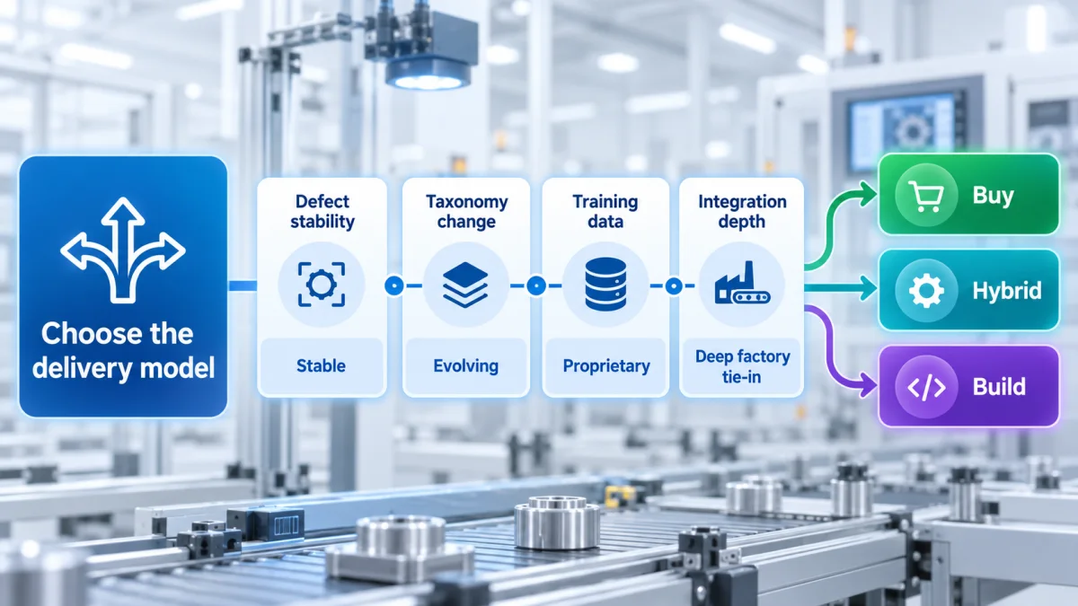
Fig 13 – Buy, Build, and Hybrid Decision Matrix

Three decision factors carry most of the weight.

1. Whether the defect class is well served by the commercial platforms available in the market.
2. Whether the taxonomy will evolve over the next 3 to 5 years or stay fixed.
3. Whether the training data is proprietary and non transferable, which pushes toward build.

Cost typically lands as a downstream consideration, since the operational cost of a poorly matched system runs higher than the price gap between buy and build over the lifetime of a program.

The technology surface and the buy versus build decision together shape the engineering scope. The application on the line shapes what that engineering has to produce.

Real World Applications in Manufacturing

Computer vision defect detection lands in different manufacturing contexts with different characteristic problems. Seven application classes recur across engagements. Cognex maintains a broader application catalog that extends these categories with additional working references, including welding inspection, glue bead inspection, seal integrity, and material quality checks.

Each application in more depth.

PCB Inspection

Printed circuit board inspection covers solder defects (bridges, cold joints, insufficient solder), component presence and orientation, silkscreen quality, and surface defects on the board substrate. The imaging challenges include reflection off metallic pads and traces, and the small physical scale of the defects relative to the board area. Object detection and segmentation both apply, often against controlled lighting rigs designed to suppress reflections at the frame level. Multi angle capture is common for solder joint inspection, since a single top down frame does not reveal joint side profile.

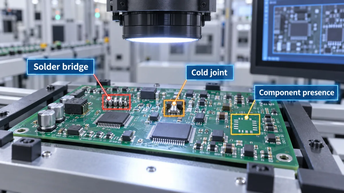
Fig 14 – PCB Inspection With Detected Solder Defects

Assembly Line Cap, Label, and Fill Checks

Bottled and packaged product lines require inspection for cap presence and orientation, label placement and alignment, seal integrity, and fill level. These are typically high volume, well defined, and stable geometry problems. Rule based image processing handles a large share of these checks reliably, with supervised classification stepping in for the categories where the acceptable variation runs wider than a simple threshold captures. Line speed drives most of the engineering effort, which typically lands on strobe lighting and global shutter cameras timed to the conveyor pitch.

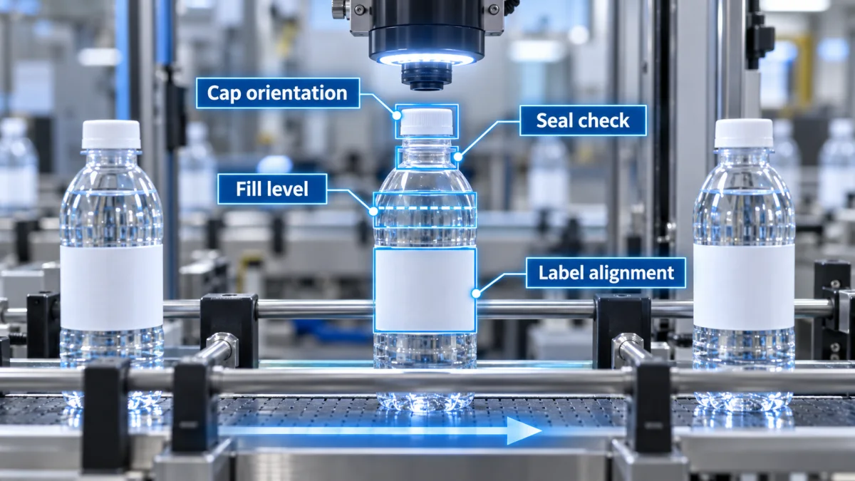
Fig 15 – Assembly Line Cap, Label, and Fill Inspection Station

Textile and Web Material Inspection

Continuous web materials including textiles, films, coated paper, sheet metal, and printed webs require line scan camera setups and segmentation models tuned for defect area and shape. Common defect categories include holes, stains, weave irregularities, coating variations, and printing errors that appear as pixel level anomalies across the surface. The engineering emphasis lands on lighting uniformity across the line and on the anomaly detection approach, since defect examples are typically rare against the volume of good material.

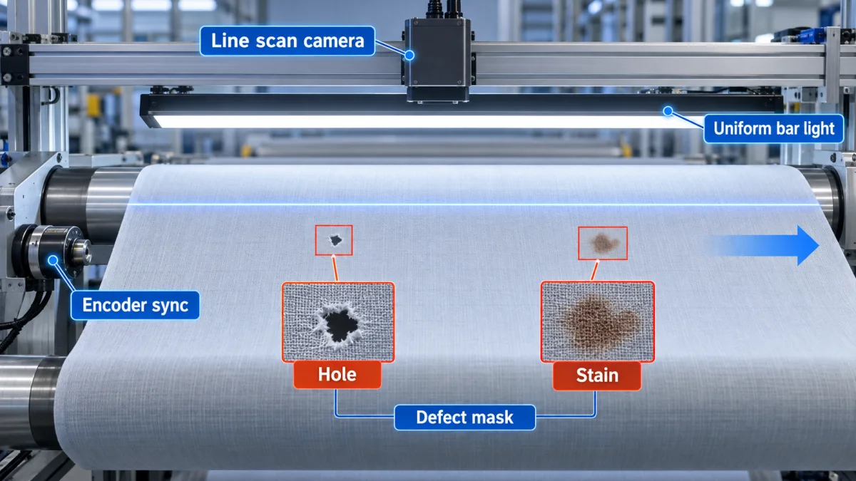
Fig 16 – Line Scan Inspection on a Continuous Textile Web

Print Anomaly Detection

Industrial printing on packaging, labels, and finished goods requires inspection for missing ink, color shift, misalignment, streaking, and character legibility. The problem class fits segmentation and anomaly detection well, with reference frame comparison as a valid rule based approach when the print target is fixed. Print defects are often subtle and require higher resolution imaging than the human eye needs to catch equivalent defects. The dashboard dimension that typically surfaces the most useful signal here is print head identifier, since streaks and missing ink often trace back to a specific head that needs cleaning or replacement.

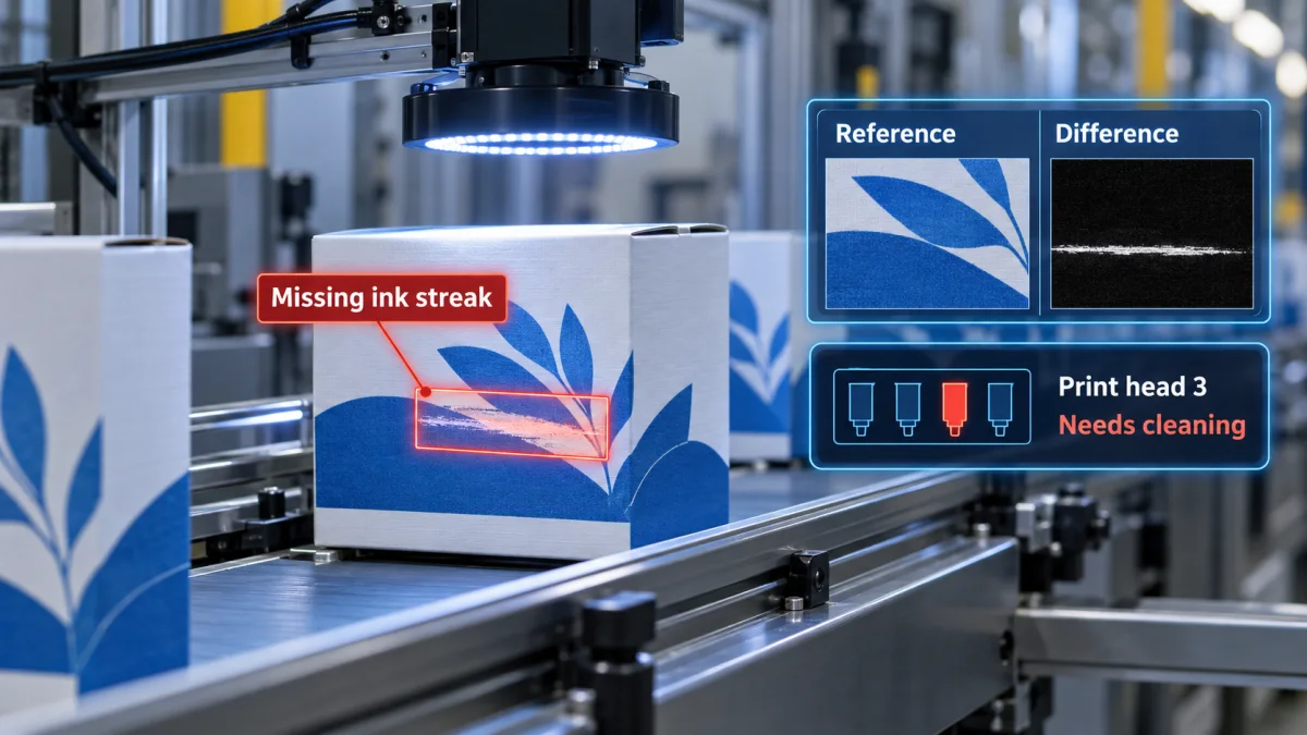
Fig 17 – Print Anomaly Detection With Print Head Attribution

Small Part Inspection

Zippers, fasteners, precision hardware, and other small parts require imaging at pixel per millimetre densities well above the typical line inspection setup. The smallest defect the operator wants surfaced runs to a fraction of a millimetre, which pushes the camera math toward high resolution sensors and short working distances. Multiple views per part are common, since small defects can hide on faces the camera does not see from a single angle. Handling and presentation systems become part of the imaging design, since the part has to arrive at the camera in a repeatable orientation.

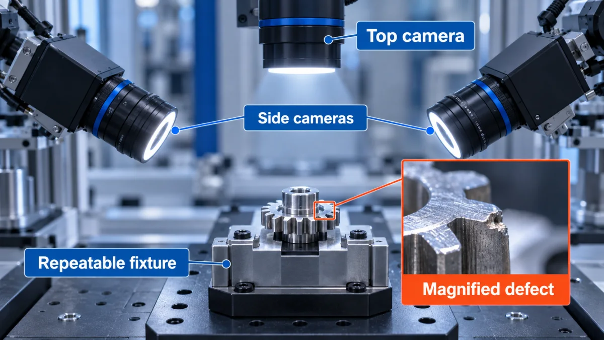
Fig 18 – Small Part Inspection With Multi Angle Capture

Coating and Enamel Pinhole Detection

High value coated goods (enamel cookware, coated automotive parts, painted architectural products) carry pinhole defects that are individually tiny and economically consequential, since a single pinhole can render a unit unsellable. The problem class fits anomaly detection well, with two stage systems adding a verifier to distinguish real pinholes from surface texture that resembles them. Imaging typically uses directional lighting to make pinholes cast visible shadows the detector can read, since a flat frontal light source can wash the pinhole out of the frame entirely.

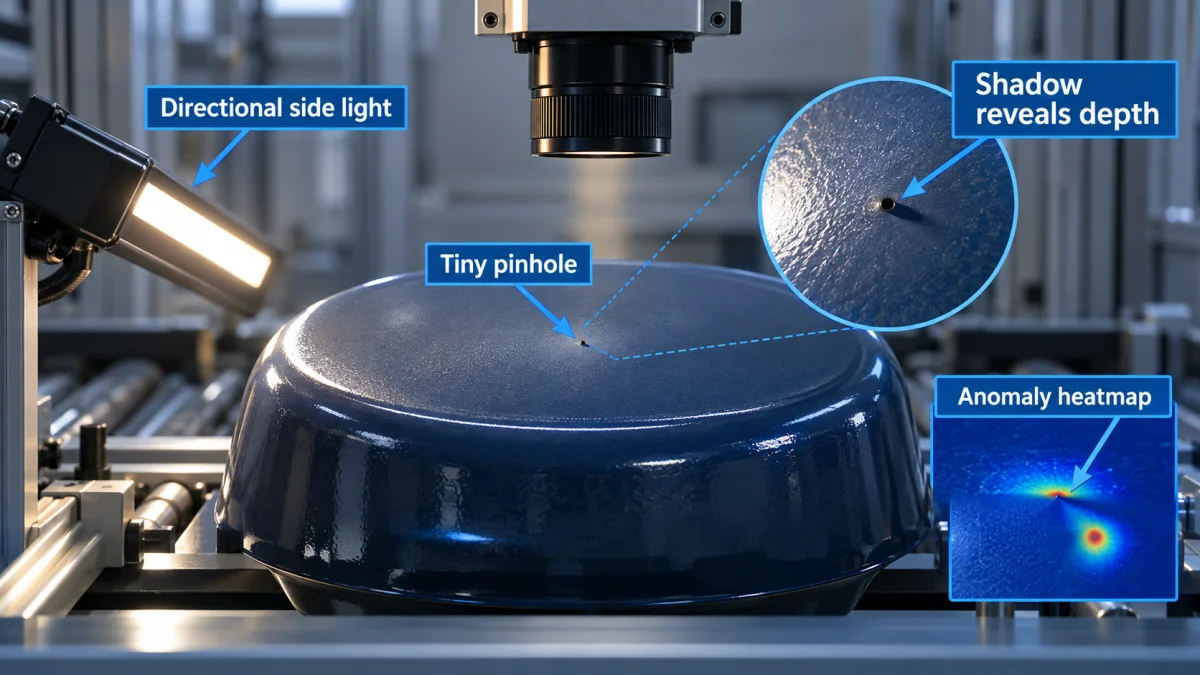
Fig 19 – Pinhole Detection on Enamel Coating With Directional Lighting

Supplier Quality Control on Incoming Goods

Inspection on incoming goods from suppliers extends the same discipline to quality gates that sit before production begins. The engineering setup can be identical to line inspection, with the difference sitting in the dashboard dimension. Findings group by supplier, batch, and product variant to surface systemic supplier quality issues that a per unit inspection does not, and the resulting data supports supplier scorecarding and contract renegotiation conversations that a subjective quality assessment cannot ground.

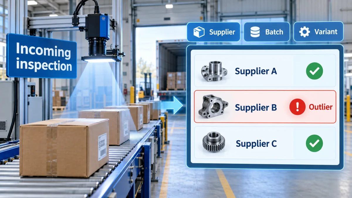
Fig 20 – Supplier Quality Control Inspection With Grouped Dashboard

The application decides the imaging, the algorithm, and the deployment shape. With a clear match between the application and the engineering approach, the remaining decisions become about handling the specific failure modes each class produces.

Where These Systems Struggle, and How Teams Fix It

Engineering honesty on defect detection systems requires naming the field failure modes and the fix for each. Six conditions recur across engagements.

Each condition in more depth.

Low Light Frames Produce False Positives on Surface Texture

Interior views, night shift lighting, and any product photographed under mixed sources produce underexposed frames where surface texture becomes visually indistinguishable from staining, cracks, or wear. A model trained only on well lit imagery raises false positives on these frames because the boundary between texture and defect is compressed by the low exposure.

Two coordinated fixes address the condition. Augmentation of the training set with underexposed samples teaches the model to read low light frames without inferring a defect from ambiguous surface texture. A capture side preprocessing step flags the operator when a frame’s exposure profile sits below a defined threshold, and suggests a retake before the frame enters inference. The Australian inspection engagement measured a reduced false positive rate on low light photos after the augmentation and retake flow entered production.

Reflective and Wet Surfaces Read as Apparent Features

Chrome, painted metal, glass, polished plastic, wet product, and reflective ground all create apparent features in the frame that the detector reads as candidate defects. The problem is worst where the reflection sits inside the product silhouette.

Two fixes coordinate here. Background segmentation removes the ground reflection and workshop clutter before the detector reads the frame, which handles the reflection outside the product silhouette. Adaptive exposure normalization reduces the glare artifact on typical frames, and frames past a reflection threshold route to retake. The salvage vision engagement combined both against wet tarmac and low sun angle glare on chrome, with routing to retake as the terminal fallback for frames that could not be normalized.

Occlusion Produces Missed Defects or Misread Frames

Snow, ice, salt, dust, packaging film, protective wrap, dirt from prior processing, and operator hands all occlude parts of the product surface in ways that either mask a real defect or produce apparent features that are not defects. The condition is universal enough that occlusion warrants an explicit detection step.

The fix is to treat occlusion as an output class of the quality classifier, which runs before the defect detector. Frames flagged with occlusion above a threshold route to physical clearing, repositioning, or retake before downstream inference. The salvage engagement handled snow and salt this way. Manufacturing setups handle packaging film and dust the same way.

Overstated Severity From Limited Evidence

A single frame cannot reliably assign cause. A dark stain is observable. Whether that stain reflects water damage, spilled coffee, or a shadow patch from a moved object cannot be resolved from the image alone. Models that produce urgent severity on visually ambiguous findings overstate the significance of what the evidence actually supports, which erodes operator trust faster than false positives do.

Three coordinated changes address the class of error. A hard negative mining pass adds confirmed non condition impacting stains and their equivalents to the training set with explicit labels. A per instance likely cause head trains jointly with the detection head, producing a coarse cause bucket per finding. A downstream postprocessing rule reads the likely cause bucket and adjusts the severity output. Findings with a cosmetic mark consistent bucket receive a not urgent severity by default. Findings with insufficient evidence route to the operator at review, with a prompt to attest to the likely cause based on their in room judgment. The category label stays observable throughout. The severity claim stays anchored to what the evidence supports. This is the exact fix the Australian inspection engagement shipped for staining findings, and it transfers directly to manufacturing quality inspection where similar cause ambiguity applies to stains, marks, and surface discoloration.

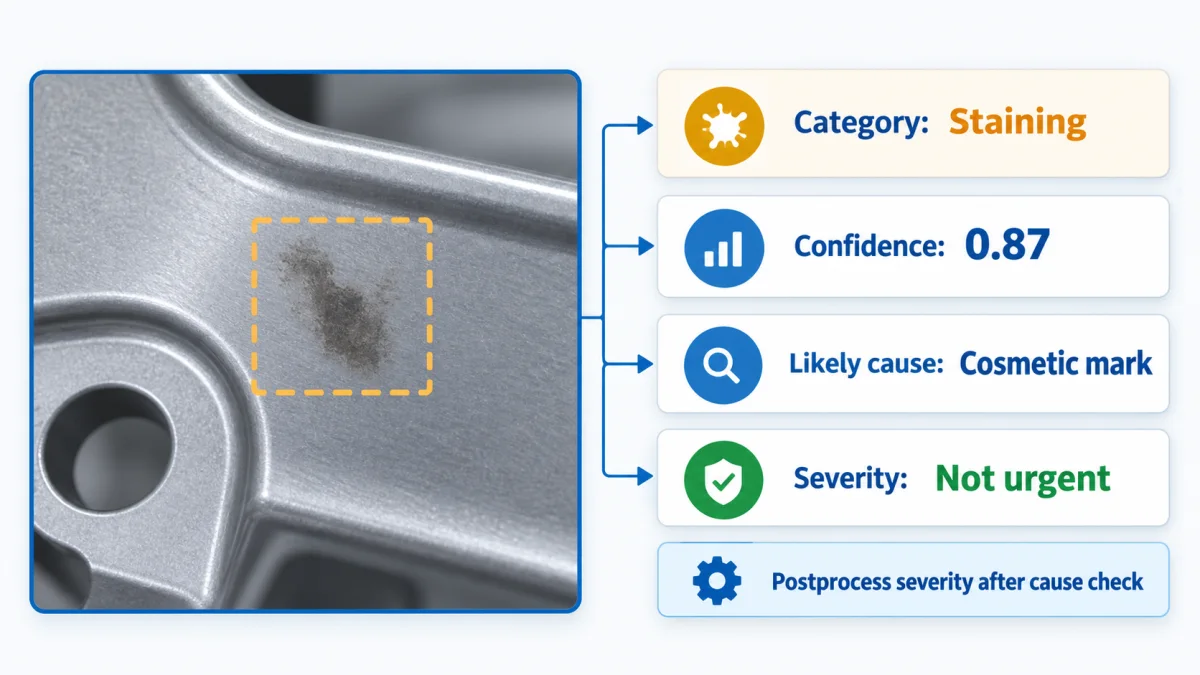
Fig 21 – Category, Confidence, and Severity Kept as Separate Fields

Class Imbalance on Rare Defects

Manufacturing programs typically have thousands of good samples and dozens of examples of the specific defect the operator wants to catch. Standard supervised training on this distribution overfits to the majority class and misses the rare event, which is the event the program exists to catch.

Two fixes apply. Anomaly detection over supervised classification is the default choice under class imbalance, since anomaly detection learns from the majority class and flags deviations. Where supervised methods are required for downstream reasons, targeted oversampling of the defect class combined with hard negative mining on visually similar non defects produces a more usable model than naive supervised training on the raw distribution.

Drift Across Shifts, Suppliers, Batches, and Seasons

Production environments change. Lighting drifts across daylight and shift transitions. Suppliers change and their product surface finish shifts with them. Batches carry variation the trained model has not seen. Camera hardware refreshes change the pixel profile. Any of these changes can shift the model’s inference distribution enough to move accuracy without triggering an obvious alert.

The fix is monitoring on inference distributions and reviewer correction rates. When the distribution of confidence scores shifts, or the correction rate on a specific category climbs, the operations team investigates the source and either recaptures training data for the shifted condition or adjusts thresholds. Model versioning and shadow evaluation let the response run without pulling the system offline.

The fixes take shape over iteration. A structured sequence for the first program makes the iteration converge faster.

An Implementation Roadmap

Ten steps carry a computer vision defect detection program from empty to production. The steps run in order for most first programs.

1. Define the defect categories, the acceptable variation, and the borderline cases in writing. Ambiguity in the definition compounds through every subsequent step.
2. Run the camera math from the smallest defect backwards to sensor, lens, and lighting. Model accuracy on a defect the camera cannot resolve is capped at zero.
3. Build a stable image capture station and hold its variables constant. Camera, lens, lighting, distance, angle, and product presentation stay fixed across the program.
4. Collect representative imagery across shifts, suppliers, batches, and lighting conditions, including hard negatives. The training corpus decides more of the outcome than any subsequent decision.
5. Establish a labeling program with a versioned taxonomy and a senior reviewer on the definitional boundaries. Per instance bounding regions, category labels, and severity tokens require dedicated labeling capacity.
6. Start with a baseline approach matched to the defect character and the data available. Anomaly detection under class imbalance, supervised methods with a bounded taxonomy and enough labeled data, rule based image processing where a threshold suffices.
7. Measure precision, recall, F1, mAP or IoU where applicable, and false alarms per 1,000 parts. Publish the baseline. Accuracy alone does not carry the actual signal on rare defect programs.
8. Run a controlled pilot alongside human inspection. Parallel operation for the first quarter or first defined observation window builds the confidence data to move human review to a smaller sample.
9. Integrate the pipeline with the factory line. PLC trigger and result contracts, image queue, worker pool, physical reject mechanism, dashboards, recipe switching, and degraded mode behavior.
10. Monitor inference distributions and correction rates for drift, and iterate model and threshold in shadow mode before promotion. Shipping is measured across the first year of operation, past the initial go live event.

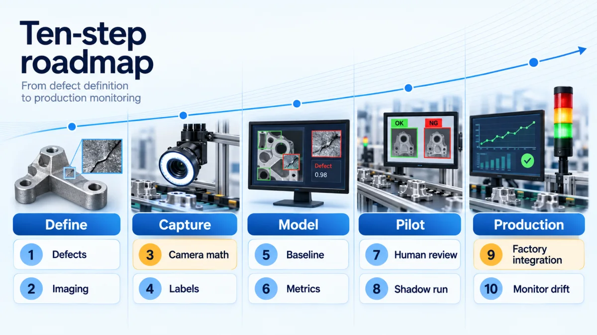
Fig 22 – Ten Step Implementation Roadmap

Ten steps carry a program from empty to production. The corrective action loop covered next extends the value the operations team can unlock from the detection data.

From Detection to Corrective Action

Detection alone produces alerts. The corrective action loop turns those alerts into process improvement, and the economic case for a defect detection program usually rests here.

The loop has five steps.

1. Group findings by dimension. Every finding writes to the quality register with machine identifier, supplier identifier, shift, batch, product variant, process step, and timestamp attached. Grouping by any of these dimensions surfaces defect concentration that a raw defect count does not. A 2 per cent defect rate that concentrates on a single machine, a single supplier’s batch, or a single shift’s handover reveals a different corrective action than a 2 per cent rate distributed evenly across the population.

1. Apply SPC methods to the grouped data. Statistical process control provides the tools for reading manufacturing data at signal versus noise resolution. Run charts show the defect rate against time and surface trends. Control charts show whether the process is operating inside its statistical bounds or shifting. Pareto charts show which defect categories carry the largest share of the total defect count, which supports prioritization on the categories that matter most to reduce.

1. Run root cause investigation on the signals SPC surfaces. The 5 whys method walks back from an observed defect concentration to its process origin through iterative why questioning. The fishbone diagram (also called Ishikawa) sorts candidate root causes by dimension, typically machine, material, method, measurement, environment, and personnel. Correlated variable analysis on the quality register data surfaces process variables that move together with the defect rate.

1. Change the process based on the identified cause. A supplier change, a machine parameter adjustment, an operator training update, a materials handling change, a maintenance schedule change. The change is a physical action on the process.

1. Verify the change on the same dashboard the detection produced. The defect rate on the affected dimension should move after the process change. If it does not, the identified cause was wrong or the change did not address the actual cause. The loop runs again.

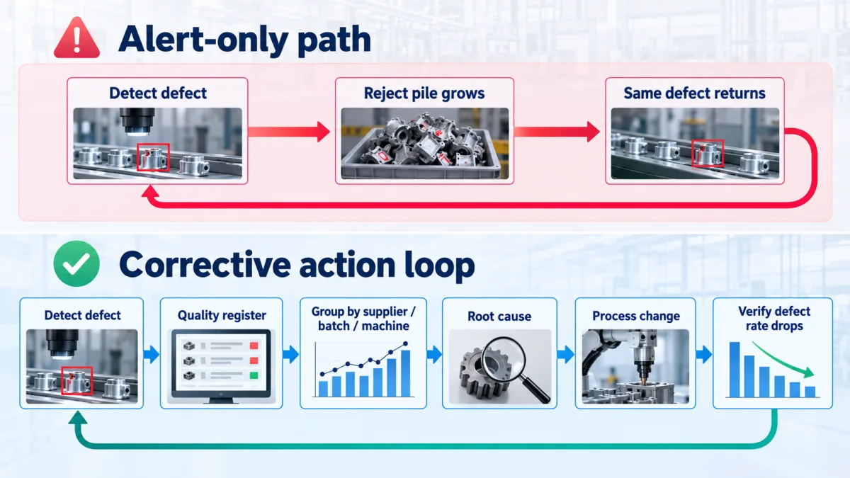
Fig 23 – The Corrective Action Loop

A defect detection program that does not close the corrective action loop produces alerts and reject piles. A program that does close the loop reduces defect rates over time and pays back its investment through fewer defects reaching finished goods.

Closing

Computer vision defect detection is an engineering discipline that touches capture hardware, model architecture, labeled data, factory integration, and operator workflow. The technology decisions that produce reliable systems are decisions about imaging, data, and the human review architecture around inference. The model choice sits inside that surrounding system.

The two engagements referenced in this read demonstrate the discipline at production scale. The Northern European salvage vehicle auction vision engagement demonstrates the multi model specialization decision, the background segmentation and occlusion handling that let the system operate through Northern European autumn and winter field conditions, and the confidence threshold calibration discipline that moved measurable operational metrics after a shadow mode evaluation. The Australian property inspection engagement demonstrates the labeling program that produced more than 350,000 individually labeled defect instances against a versioned taxonomy, the downstream fine tuned reporting classifier over the detection head, the hard negative mining approach to overstated severity, and the room level human review gate that outperformed end of workflow review.

Manufacturing quality inspection carries the same underlying engineering discipline. The vocabulary shifts from adjusters and inspectors to line operators and quality engineers. The surrounding decisions run the same way.

Talk to Clixlogix About a Defect Detection Program