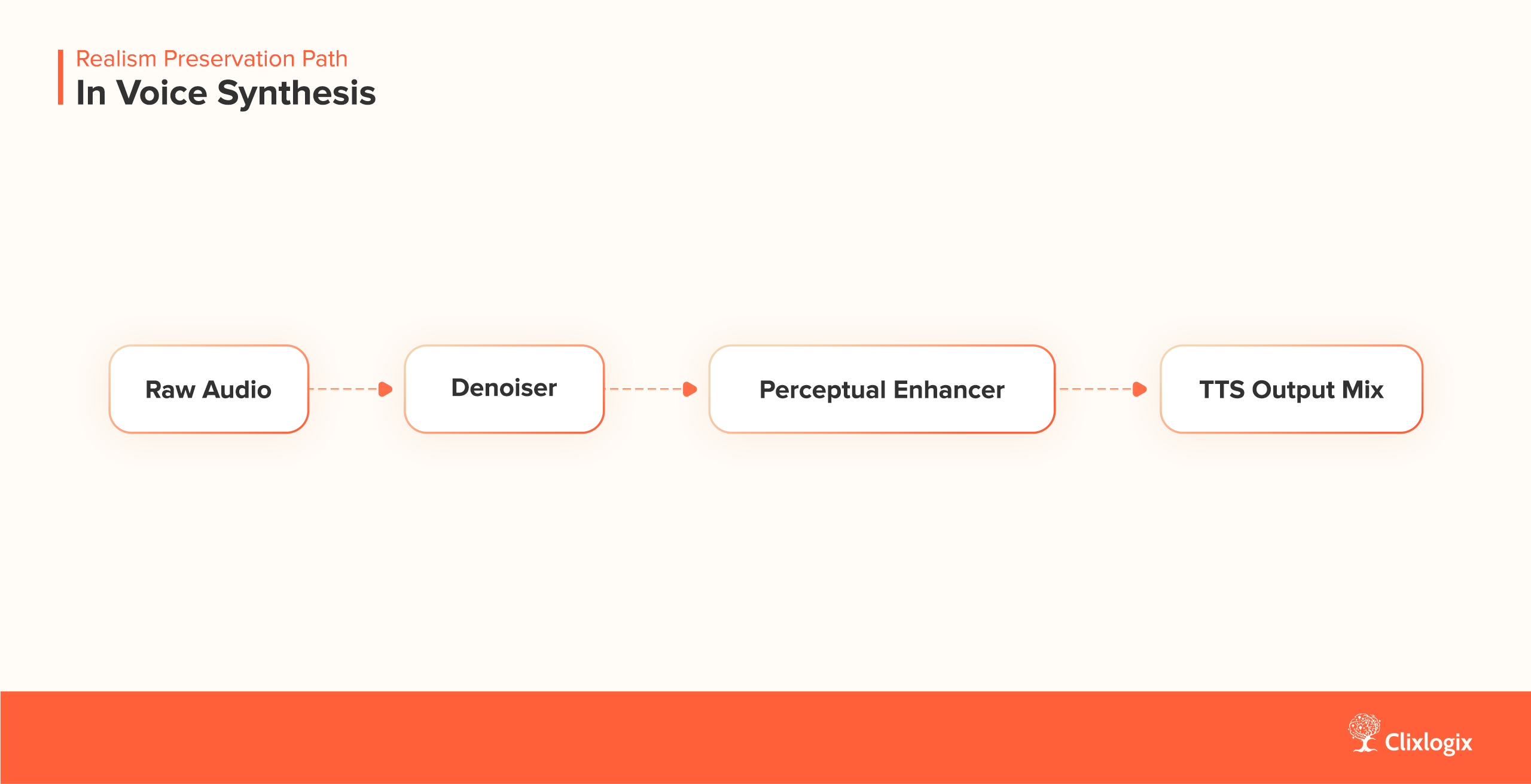
Participants consistently rated the mixed/noisy-trained model higher in presence and prosody continuity, describing it as “less robotic” and “more natural in pauses.” Objective SNR analysis confirmed higher robustness: degradation < 5 % MOS under 12 dB ambient noise, versus 15 % for the clean-only model.
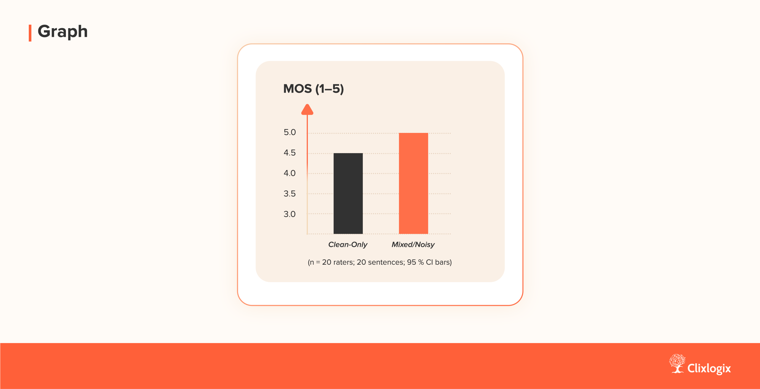
These results align with prior literature (e.g., Valentini-Botinhao et al., SSW 2016), supporting the hypothesis that modest noise exposure during training enhances generalization and perceived realism in synthetic voices.
Beyond our simulated MOS comparison, the BASE TTS team reported similar human-rated gains as model size increased. Linguistic experts evaluated ‘small,’ ‘medium,’ and ‘large’ configurations on seven expressive dimensions. Larger models consistently scored higher on compound nouns, punctuation, questions, and syntactic complexity, confirming that scale improves prosody, pacing, and semantic retention.
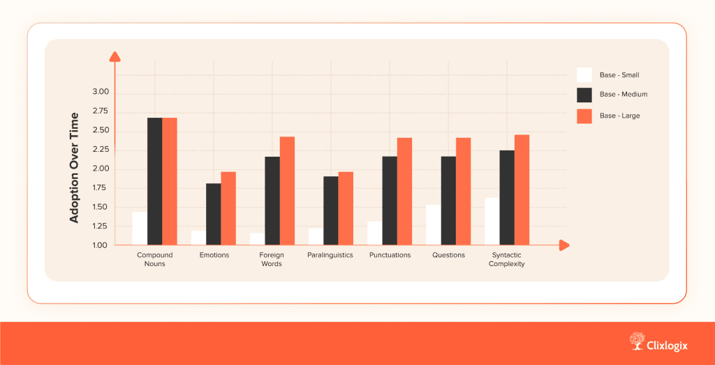
Figure 5: Mean expert scores across linguistic dimensions show scaling benefits for BASE TTS models (source: BASE TTS, arXiv 2402.08093)
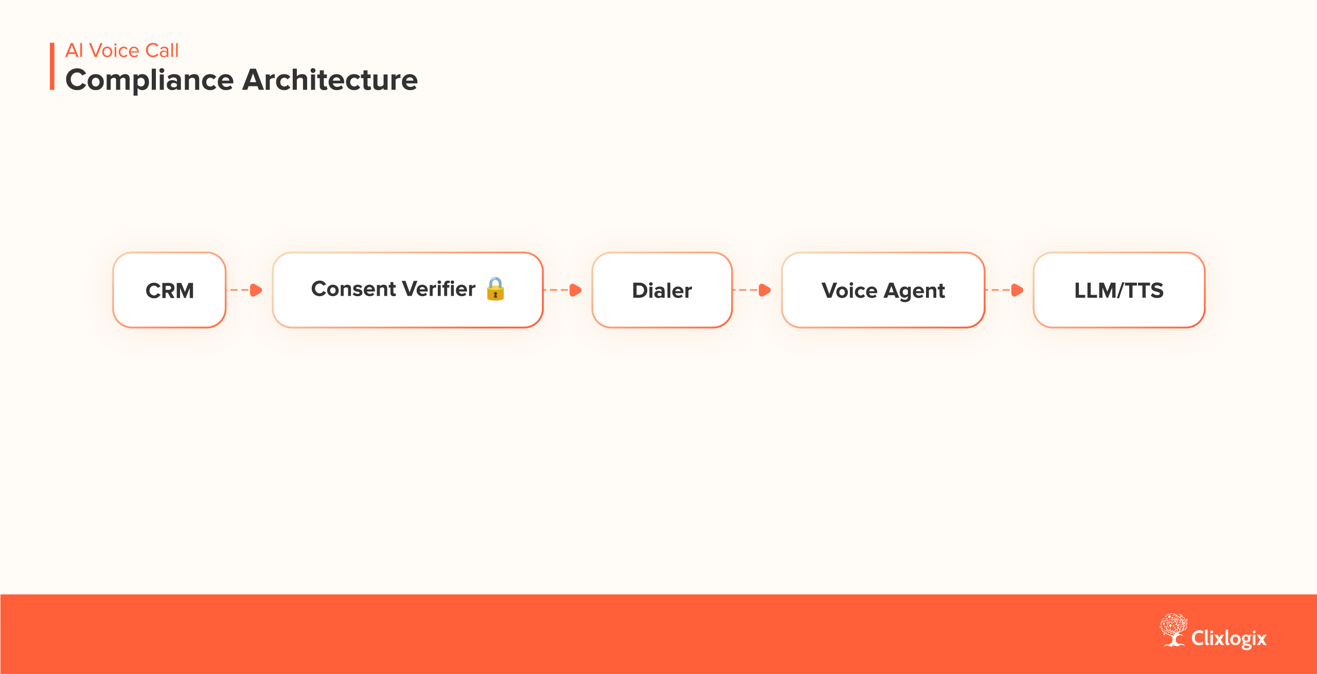
Architectural Patterns for Robustness
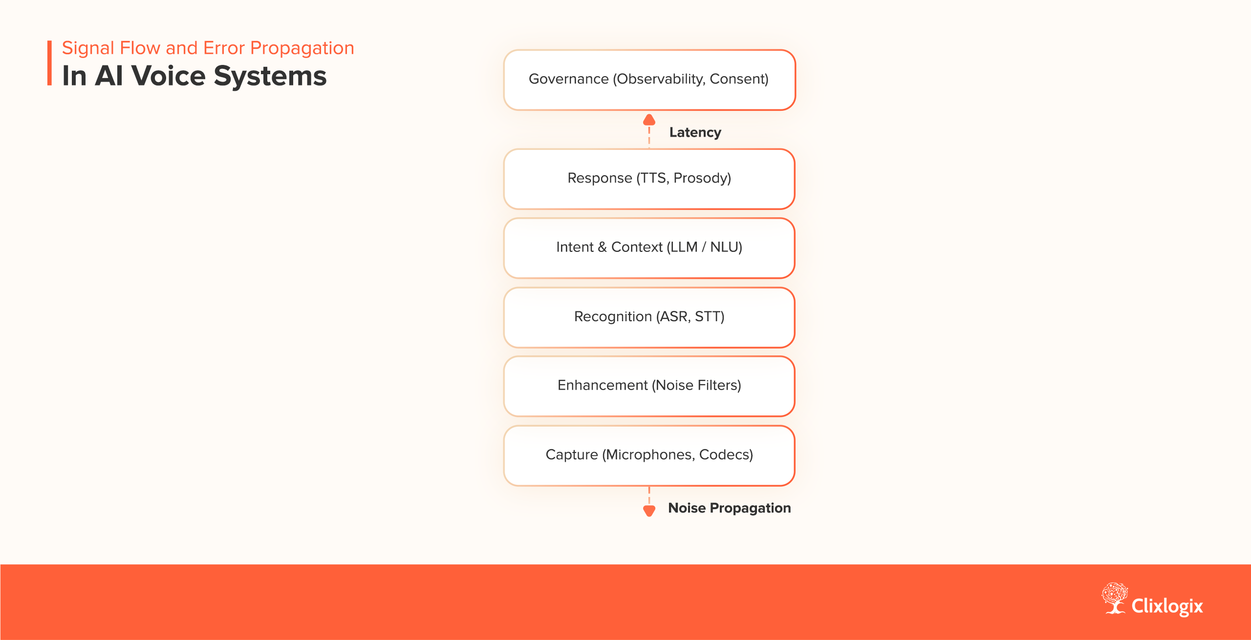
Noise is not a single fault but it is a distributed constraint. Robust systems respond by placing control at multiple points in the chain. Each pattern below defines where that control lives and what trade-offs it introduces.
1. Edge Enhancement – Performs noise suppression locally to prevent transmitting raw interference. Common approaches use WebRTC acoustic echo cancellation (AEC) or RNNoise filters. This reduces uplink bandwidth and stabilizes performance on weak networks but depends on hardware variability, as mobile DSP chips follow different suppression curves.
2. Media Proxy – Acts as a middle layer that performs normalization and suppression before ASR, ensuring consistent input quality across devices. This provides uniform model performance regardless of client source but introduces an additional 50–80 ms of latency per round trip.
3. Dual Channel Confidence – Runs ASR on both the raw and enhanced audio streams, then merges their confidence scores using threshold logic. This improves reliability under intermittent noise conditions but adds around 10–15 % CPU load.
confidence = max(raw_conf, enhanced_conf)
if abs(raw_conf - enhanced_conf) > 0.3:
flag_for_review()
4. Adaptive Turn Taking – Combines voice activity detection (VAD) with token-stream awareness so that agents can recognize natural pauses and yield control mid-sentence. This pattern improves conversational flow and minimizes overlapping speech, creating a more natural dialogue rhythm.
if vad.detect_silence(duration=350ms):
agent.speak_next_token()
5. Graceful Degradation – Switches to text-based channels when ambient noise surpasses a defined threshold. Commonly applied in 24/7 AI receptionist workflows, this pattern maintains continuity even under poor acoustic conditions by routing interactions through SMS or chat interfaces.
if snr < 10:
switch_channel('sms')
6. Telemetry Loop – log SNR, ASR confidence, and retry count for retraining.
Force: continuous model improvement.
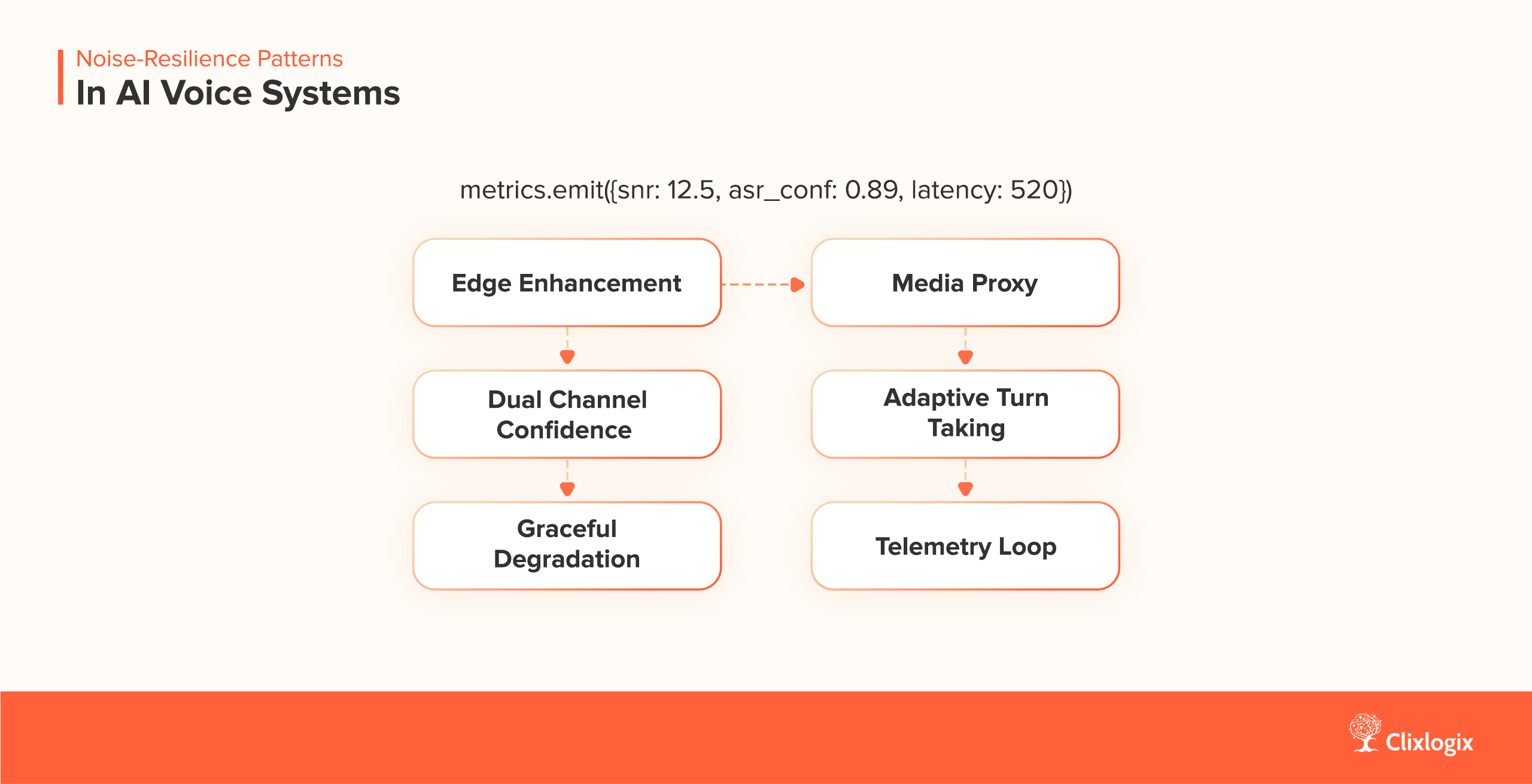
Figure 6: Noise-Resilience Patterns in AI Voice Systems.
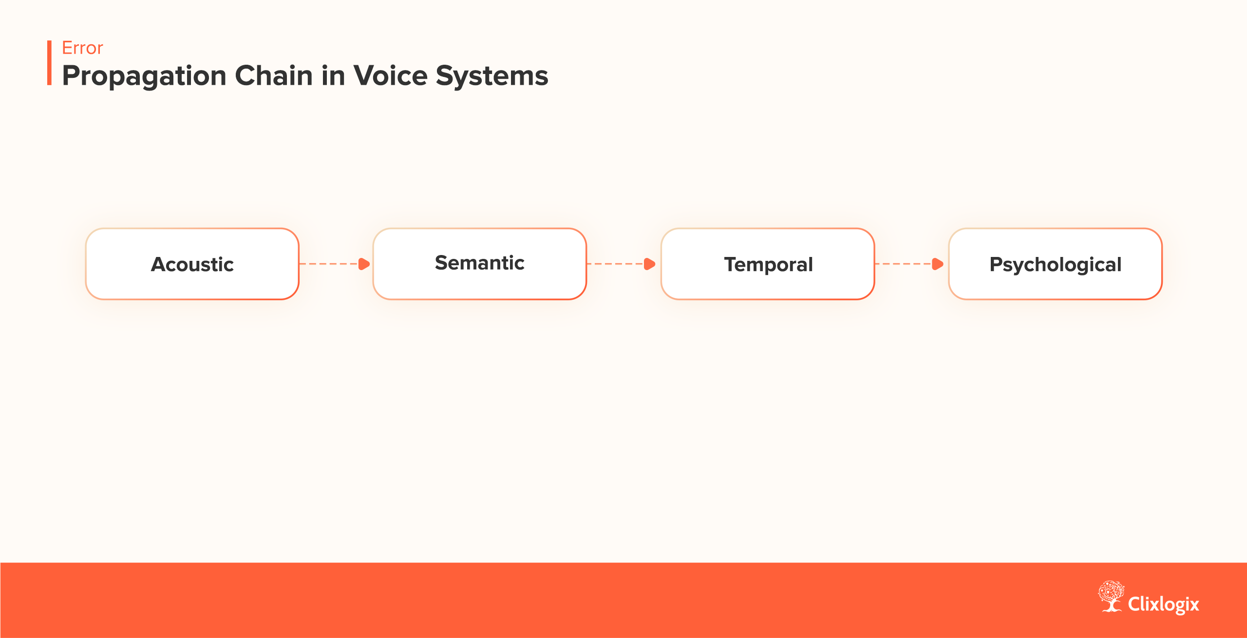
Each of the above pattern controls where noise is handled, edge, proxy, or model loop, creating a distributed surface that balances clarity, latency, and resource cost. These patterns together form the “noise resilience surface” of a voice system.
Field Results and Real-World Scenarios
Case 1 – 24/7 Appointment Line, U.S.
The system handled thousands of inbound calls daily, many from hospital corridors and parking lots. Initial models misfired on background announcements, marking them as patient speech. By adding a dual-channel confidence setup, one ASR stream processed raw audio while the other used enhanced input. The system compared both transcripts and chose the higher-confidence line for intent mapping. False triggers fell by 34 %, and token usage dropped 9 %.
The second ASR instance paid for itself within ten days, mostly through shorter conversations and fewer manual transfers.
Case 2 – Logistics Dispatch Line, Saudi Arabia
Dispatchers worked across warehouse yards and truck bays where engines ran constantly. An edge-based noise suppressor using 10 ms frame windows was added to Android devices before the media proxy. This local filter removed heavy engine bands without affecting speech cues. Callbacks dropped by 18 %, and round-trip latency stabilized under 550 ms even on cellular links.
The change shifted troubleshooting time from “bad audio” to “route mismatch,” showing the acoustic layer was no longer the bottleneck.
Case 3 – Retail Voice Concierge, Netherland
The store’s voice concierge operated in open retail floors with constant chatter and music. Customers often overlapped the agent’s speech, forcing restarts. Adaptive turn-taking logic combined voice-activity detection (VAD) with token streaming, teaching the agent to pause when human speech resumed. Conversation overlap fell by 22 %, and perceived response speed improved even though the underlying large language model (LLM) and text-to-speech (TTS) stack stayed the same.
The gain came purely from timing discipline.
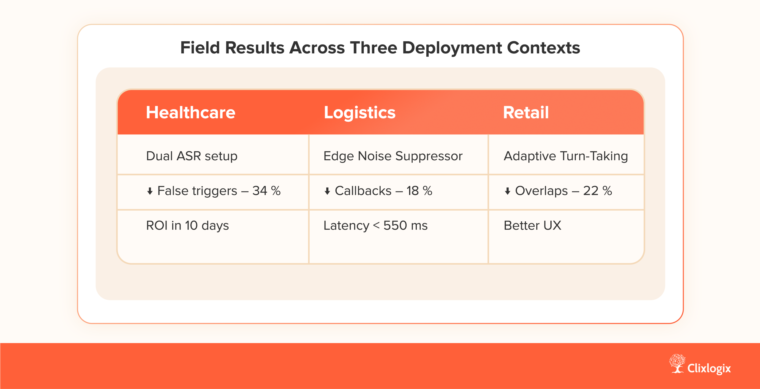
Figure 7: Field Results Across Three Deployment Contexts
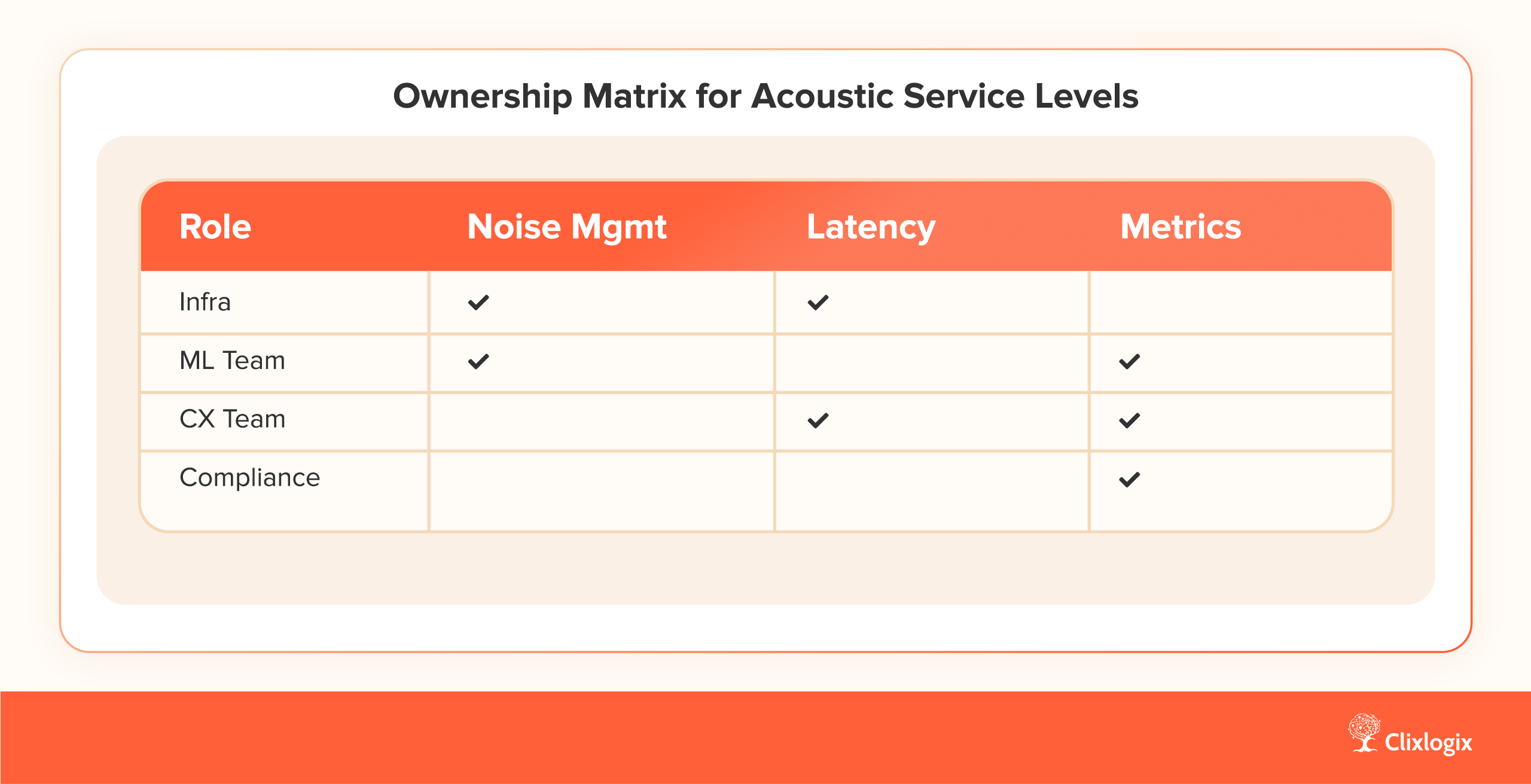
Observability & Monitoring
Voice systems require observability beyond standard metrics. Teams should track acoustic and semantic health:
- Signal metrics – SNR distribution, VAD trigger rate, silence duration histograms.
- Performance metrics – latency percentile (P95), token throughput, speech synthesis lag.
- Semantic metrics – intent match accuracy, confidence variance.
Dashboards should combine audio telemetry with system logs. A minimal SQL-style query for insight:
SELECT AVG(latency_ms), AVG(snr_db) FROM voice_events WHERE snr_db < 15;
This helps engineers identify where network or microphone quality degrades user experience. Modern pipelines integrate Prometheus exporters to visualize these metrics in Grafana.
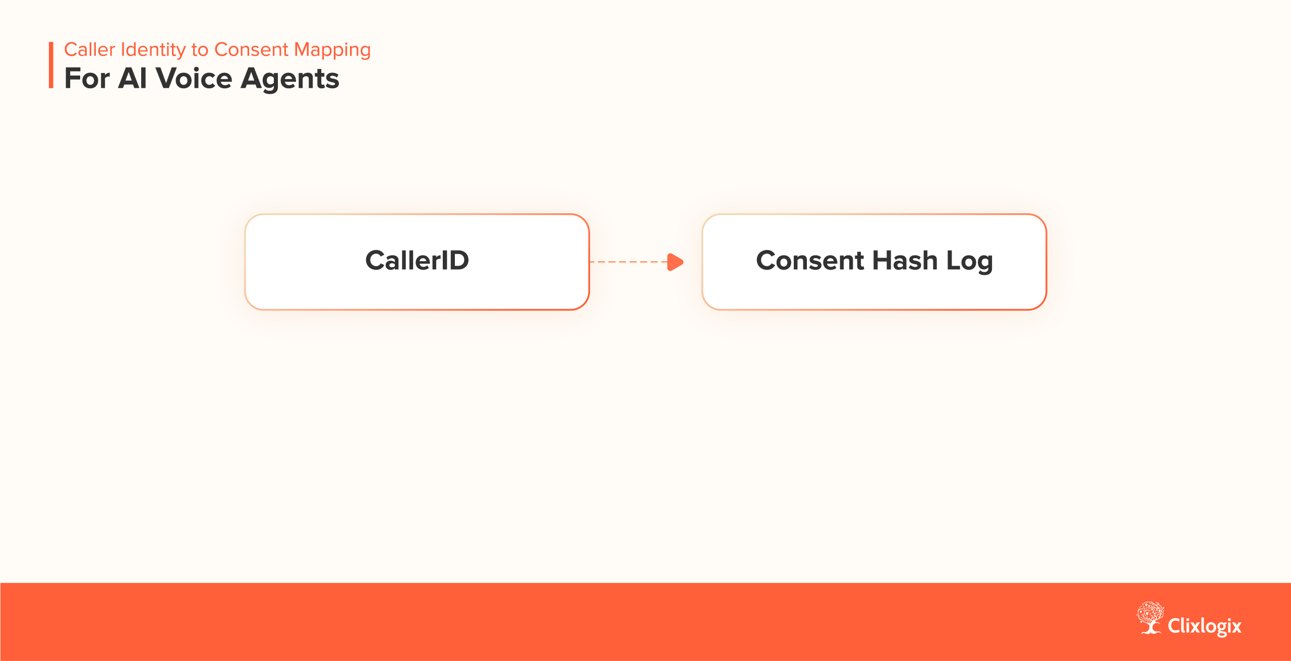
Monitoring should extend to consent logging and ASR transcript anomalies. Observability closes the loop between architecture and behavior.
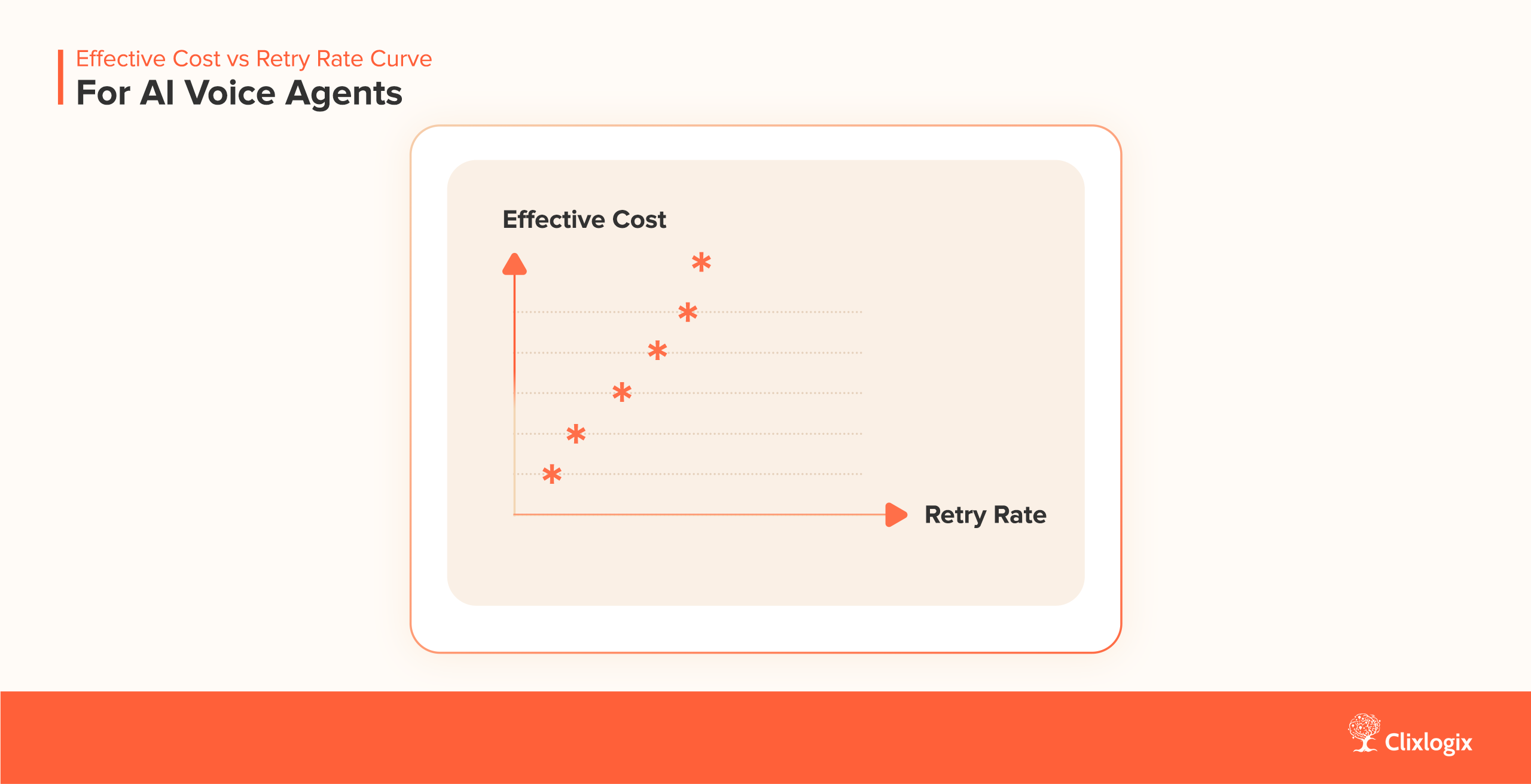
Noise Budgeting in Design Reviews
Teams often allocate milliseconds and megabytes; few allocate decibels. A noise budget defines how much degradation each layer can tolerate before cascading failure.